Coursework | November 2024
Poisson Image Editing
Image Processing by Prof Lourdes Agapito
University College London (UCL)
Fig. 1. Poisson image editing allows to seamlessly clone a region from image A in image B. In this example we transfer a face into the
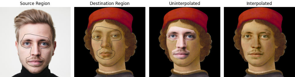
"Portrait of a Youth" [1]
During my MSc in Computer Graphics, Vision and Imaging I was lecturing a module about Image Processing in which one of my student projects focused on Poisson Image Editing. It is a seamless cloning method to transfer and interpolate a frequency pattern from an arbitrary image into another solving a poisson equation for each pixel to clone. The method was first introduced by
Perez et al. in 2003. [2]
Method
We will mainly focus on guided image interpolation, which in simple terms adjusts the image intensities over region Ω such that their gradient matches a reference gradient. This optimization is in a way separated from the color itself and alters the image on a more abstract level by remodelling the "curvature" of its intensities.

All we need is a destination image D with region Ω in which we want to clone the region Ω from a source image S described by its vector field v, capturing the gradience. In theory one could come up with any v without requiring S, however we will stick to it for clarity.
Figure 2: The destination image can be described with the function f. Within f we have the interpolation region Ω which is represented with function f and solved for under the guidance of vector field v and given the dirichlet boundary condition δΩ. In this example vector field v is the image gradient for S within the corresponding region Ω.
Minimizing the difference between f and v for all pixels p in region Ω can be rewritten with the following poisson equation while using a dirichlet boundary condition to ensure seamless cloning. The laplacian Δ allows us to measure the local difference of a point and in our case the difference between the intensity of a pixel p to its neighbours.
Δf=Δg over Ω, with f|δΩ=f|δΩ
This gives us a linear system to solve for all pΩ. One can think of the below equation as some extended form of the laplacian operator to solve the minimization problem for region Ω.
|Np|fpqNpΩfq=qNpδΩfq+qNpvpq
Np = Number of neighbours
p = Pixel
fq = Neighbouring pixel
Ω = Region to interpolate
δΩ = Boundary of region to interpolate which is static and belongs to f
f = Region of function to interpolate
f = Destinatination image function outside of region
v = Vector field
Figure 3: On a higher level the interpolation remodels the region Ω of D in such a way that it is as close a possible to Ω of S but blends smoothly into the curvature of f.
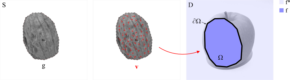
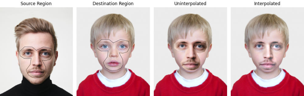
Following the method described above there are two ways to apply it for seamless cloning in images: (i) importing the gradient solely from the source image and willing to remove any details in region Ω from the destination image (ii) mixing the gradients of source and destination over Ω by maintaining the highest frequencies from both images and preserving ultimately detail.

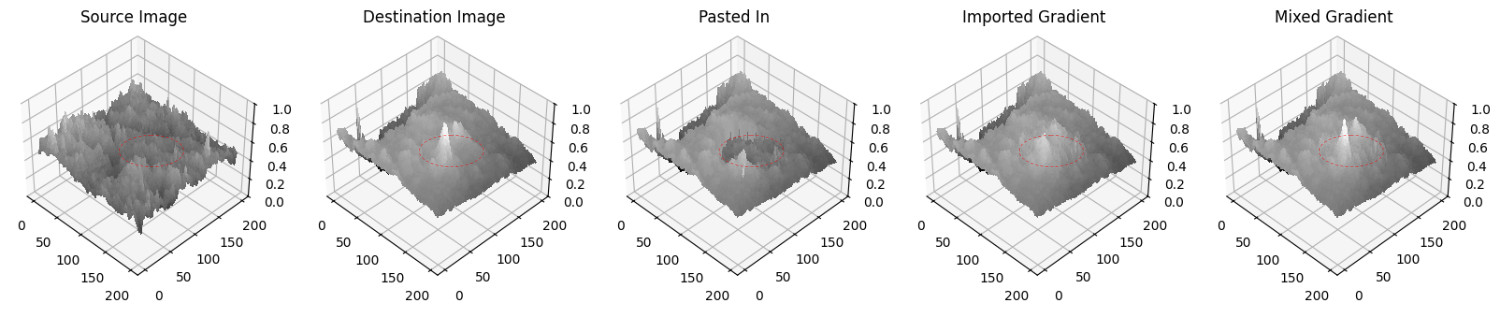
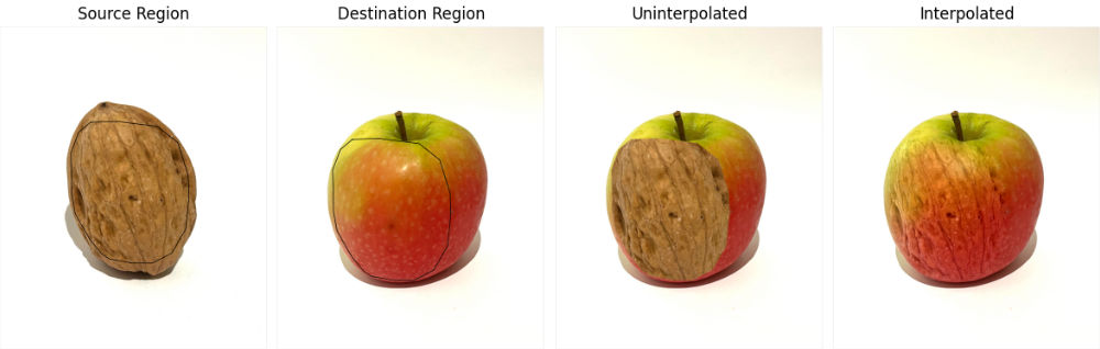
In figure 3 this becomes particularly visible when comparing the specular reflections on the apple in the images but especially comparing the gradients. When importing the gradient this reflection gets blurred, when mixing it is preserved. On the other hand we showcase for reference how Ω would look like if it would be just pasted in the destination and not interpolated, creating high, unnatural looking frequencies at δΩ.
Figure 4: Seamless cloning of a region on a walnut to an apple in greyscale to simplify the problem to a single image channel. The light red dashed line highlights the region Ω in the source and destination image which was transferred.
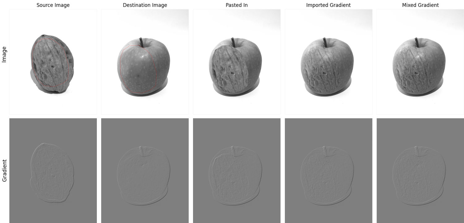
So far the example was only a grayscale image. For multi-channel images one has to solve the above minimization problem for each individual channel independently. Figure 5-8 showcase this on the example of trasnfering the texture of a walnut onto an apple in RGB.
Figure 5: Red channel interpolation.
Figure 6: Green channel interpolation.
Figure 7: Blue channel interpolation.
Figure 8: Stacked interpolated channels.
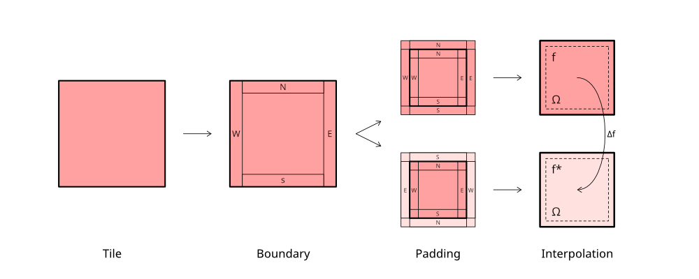
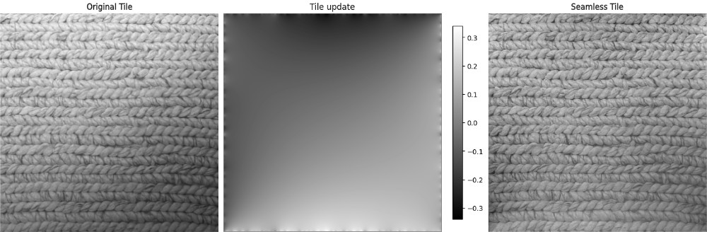
It is a widely known issue of using arbitrary images as textures for 3D models that by populating the geometry with the texture tile they create visible tiling seams which are not desired. Poisson image editing can be used to synthesise a seamless texture tile from any texture. With the above technique it is possible to take some arbitrary image and create a ‘tiling’ boundary condition δΩ by mirroring the edge conditions, such that when solved for one removes the tiling seam.
Figure 9: Seamless tiling takes any given image and creates a source and destination image for the poisson solver. The source image is padded by offsetting its boundary, the destination image mirrors this padding SN and WE. Importing the gradience from the source image will cause the tile boundary to be interpolated into the tiling grid and ultimately blend the seam.
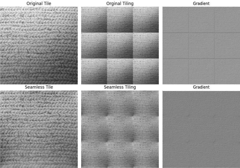
The effect of seamless tiling becomes particularly visible when applying it to a texture with big differences in illumination, given that textures mostly follow the same pattern when it comes to color and gradience. In such a case the method evenly distributes the illumination across the tile and the seam becomes nearly invisible even though the texture pattern does not match exactly. In figure 11 this illumination redistribution is made visible and indicates basically a complementary intensity to the original tile.
Figure 10: The rectangular tiling seam becomes obvious when looking at the image gradience of the tiled texture. This seam nearly vanishes after the interpolation. The corner seems to still be an issue, which might be fixed by adjusting δΩ.
Figure 11: During interpolation the original tile is adjusted in intensity to ensure smooth blending from one tile into another. The adjustment equals almost an inverted, flat illumination of the original tile.
Results
Fig. 12. Seamless transfer of face onto a foreign head.
Fig. 13. Seamless texture transfer from a walnut to an apple.
Fig. 14. Seamless transfer of an eye onto a hand.
References